Introduction
A species-area relationship (SAR) visualizes the relationship between species richness (the number of species) and the area of the land mass on which the species live. The observation that species richness increases with increasing area is a fundamental law of ecology, and a disruption in this relationship may be associated with habitat loss, habitat fragmentation, and increasing numbers of non-native species. Creating SARs for island-dwelling species helps researchers understand how trends in biodiversity across archipelagos are changing due to these effects.
The goal of this vignette is to use the SSARP R package to create a SAR for Anolis, a well-studied genus of lizards. We will focus on Anolis occurrence records from the Caribbean Islands. More information about the SSARP package and a comparison to a previously published SAR for Anolis can be found in the manuscript associated with the package.
In order to construct a species-area relationship with SSARP, we will:
- Gather occurrence data from GBIF
- Filter out invalid occurrence records
- Find areas of pertinent land masses
- Create a species-area relationship
Gathering Occurrence Data
GBIF (Global Biodiversity Information Facility) provides an easy method for gathering occurrence data for taxa of interest. SSARP uses functions from the rgbif package to gather occurrence records associated with a given taxon. The user may also provide their own data for use in creating a SAR, but we will use GBIF in this example.
In order to access data from GBIF, we must first determine the unique
identifying key associated with the taxon of interest. We will use the
SSARP::get_key() function from SSARP to obtain
this key.
library(SSARP)

# Get the GBIF key for the Anolis genus
key <- get_key(query = "Anolis", rank = "genus")

# Print key
key
## [1] 8782549Now that we have the key associated with Anolis, we will use
this key with the SSARP::get_data() function to gather
georeferenced occurrence records from GBIF. The “limit” parameter will
be set to 10000 in this case for a quick illustration of
SSARP’s functionality, but this parameter can be as large as
100,000 (the hard limit from rgbif for the number of records
returned).
We are only interested in occurrence records for island-dwelling anole lizards located in the Caribbean, so we will geographically restrict the returned data to this area by setting the “geometry” parameter to a polygon in Well Known Text (WKT) format that encompasses the Caribbean islands (Figure 1).
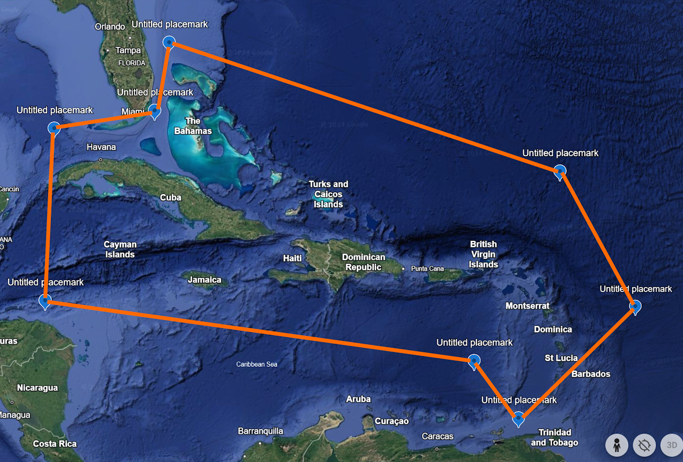
# Get data for Anolis from GBIF in the specified polygon
dat <- get_data(key = key, limit = 10000, geometry = 'POLYGON((-84.8 23.9, -84.7 16.4, -65.2 13.9, -63.1 11.0, -56.9 15.5, -60.5 21.9, -79.3 27.8, -79.8 24.8, -84.8 23.9))')

# Print first 5 lines of dat
head(dat, n = 5)
## # A tibble: 5 × 155
## key scientificName decimalLatitude decimalLongitude issues datasetKey publishingOrgKey installationKey
## <chr> <chr> <dbl> <dbl> <chr> <chr> <chr> <chr>
## 1 5007064248 Anolis distichus Cop… 19.0 -69.0 cdc,c… 50c9509d-… 28eb1a3f-1c15-4… 997448a8-f762-…
## 2 5007082681 Anolis evermanni Ste… 18.3 -66.3 cdc,c… 50c9509d-… 28eb1a3f-1c15-4… 997448a8-f762-…
## 3 5007565800 Anolis cristatellus … 18.4 -66.0 cdc,c… 50c9509d-… 28eb1a3f-1c15-4… 997448a8-f762-…
## 4 5008127474 Anolis sagrei Duméri… 18.4 -64.5 cdc,c… 50c9509d-… 28eb1a3f-1c15-4… 997448a8-f762-…
## 5 5037019266 Anolis leachii Dumér… 17.1 -61.8 cdc,c… 50c9509d-… 28eb1a3f-1c15-4… 997448a8-f762-…
## # ℹ 147 more variables: hostingOrganizationKey <chr>, publishingCountry <chr>, protocol <chr>, lastCrawled <chr>,
## # lastParsed <chr>, crawlId <int>, basisOfRecord <chr>, occurrenceStatus <chr>, taxonKey <int>, kingdomKey <int>,
## # phylumKey <int>, classKey <int>, familyKey <int>, genusKey <int>, speciesKey <int>, acceptedTaxonKey <int>,
## # acceptedScientificName <chr>, kingdom <chr>, phylum <chr>, family <chr>, genus <chr>, species <chr>,
## # genericName <chr>, specificEpithet <chr>, taxonRank <chr>, taxonomicStatus <chr>, iucnRedListCategory <chr>,
## # dateIdentified <chr>, coordinateUncertaintyInMeters <dbl>, continent <chr>, stateProvince <chr>, year <int>,
## # month <int>, day <int>, eventDate <chr>, startDayOfYear <int>, endDayOfYear <int>, modified <chr>, …Finding Land Mass Names and Areas
Once the occurrence data is returned, we will use each occurrence record’s GPS point to determine the land mass on which the species was found and find the area associated with that land mass using a database of island areas and names from SSARP.
# Find land mass names
land_dat <- find_land(occurrences = dat)

# Print first 5 lines of land_dat
head(land_dat, n = 5)
## SpeciesName Genus Species Longitude Latitude First Second Third
## 1 Anolis distichus Cope, 1861 Anolis distichus -69.010239 19.015033 <NA> <NA> <NA>
## 2 Anolis evermanni Stejneger, 1904 Anolis evermanni -66.314592 18.29657 Puerto Rico <NA> <NA>
## 3 Anolis cristatellus Duméril & Bibron, 1837 Anolis cristatellus -65.957558 18.396785 Puerto Rico <NA> <NA>
## 4 Anolis sagrei Duméril & Bibron, 1837 Anolis sagrei -64.512895 18.384578 <NA> <NA> <NA>
## 5 Anolis leachii Duméril & Bibron, 1837 Anolis leachii -61.847698 17.118499 Antigua <NA> <NA>
## datasetKey
## 1 50c9509d-22c7-4a22-a47d-8c48425ef4a7
## 2 50c9509d-22c7-4a22-a47d-8c48425ef4a7
## 3 50c9509d-22c7-4a22-a47d-8c48425ef4a7
## 4 50c9509d-22c7-4a22-a47d-8c48425ef4a7
## 5 50c9509d-22c7-4a22-a47d-8c48425ef4a7The locality information is split across three columns: “First,”
“Second,” and “Third.” The mapping utilities that SSARP uses
sometimes output different levels of specificity for locality
information (up to three different levels), so these columns provide
space for these different levels. The island name that we are interested
in will be in the last filled-in column of the three. For example, if
there are two columns of locality information for a given occurrence
record, the island name will be in the second. If there is only one
column of locality information, it will contain the island name (as with
Puerto Rico and Antigua above). If all columns have NA, the
occurrence record is invalid and will be filtered out in the next
step.
Now that we have determined the names of the land masses associated with each occurrence record, we will find the area associated with each land mass.
# Use the land mass names to get their areas
area_dat <- find_areas(occs = land_dat)

# Print first 5 lines of area_dat
head(area_dat, n = 5)
## SpeciesName Genus Species Longitude Latitude First Second Third
## 2 Anolis evermanni Stejneger, 1904 Anolis evermanni -66.314592 18.29657 Puerto Rico <NA> <NA>
## 3 Anolis cristatellus Duméril & Bibron, 1837 Anolis cristatellus -65.957558 18.396785 Puerto Rico <NA> <NA>
## 5 Anolis leachii Duméril & Bibron, 1837 Anolis leachii -61.847698 17.118499 Antigua <NA> <NA>
## 6 Anolis leachii Duméril & Bibron, 1837 Anolis leachii -61.845561 17.121707 Antigua <NA> <NA>
## 7 Anolis grahami Gray, 1845 Anolis grahami -77.060327 18.39293 Jamaica <NA> <NA>
## datasetKey areas
## 2 50c9509d-22c7-4a22-a47d-8c48425ef4a7 9710687500
## 3 50c9509d-22c7-4a22-a47d-8c48425ef4a7 9710687500
## 5 50c9509d-22c7-4a22-a47d-8c48425ef4a7 301187500
## 6 50c9509d-22c7-4a22-a47d-8c48425ef4a7 301187500
## 7 50c9509d-22c7-4a22-a47d-8c48425ef4a7 12225750000Now, our occurrence record dataframe includes records with GPS points that are associated with a land mass, along with the areas of those land masses (in m^2).
The SSARP::remove_continents() function removes any
continental occurrence records, which is useful when the user is only
interested in island-dwelling species (as we are in this example). While
the data obtained by using the SSARP::get_data() function
was geographically restricted, potential user error in specifying the
polygon in WKT format often leads to accidental continental records that
will be removed by using this function.
nocont_dat <- remove_continents(occs = area_dat)Create Species-Area Relationship
Finally, we will generate the SAR using the
SSARP::create_SAR function. The
SSARP::create_SAR() function creates multiple regression
objects with breakpoints up to the user-specified “npsi” parameter. For
example, if “npsi” is two, SSARP::create_SAR() will
generate regression objects with zero (linear regression), one, and two
breakpoints. The function will then return the regression object with
the lowest AIC score. The “npsi” parameter will be set to one in this
example. Note that if linear regression (zero breakpoints) is
better-supported than segmented regression with one breakpoint, the
linear regression will be returned instead.
create_SAR(occurrences = nocont_dat, npsi = 1)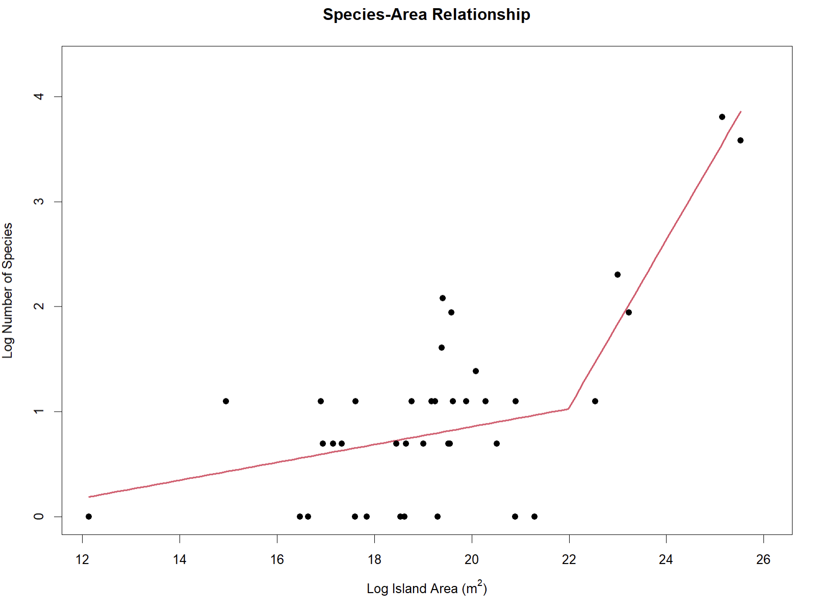
##  ***Regression Model with Segmented Relationship(s)***
##
## Call:
## segmented.lm(obj = linear, seg.Z = ~x, npsi = 1, control = seg.control(display = FALSE))
##
## Estimated Break-Point(s):
##           Est. St.Err
## psi1.x 21.977   0.75
##
## Coefficients of the linear terms:
##             Estimate Std. Error t value Pr(>|t|)
## (Intercept) -1.03529    1.00142  -1.034   0.3090
## x            0.09608    0.05355   1.794   0.0822 .
## U1.x         0.67880    0.21273   3.191       NA
## ---
## Signif. codes:  0 ‘***’ 0.001 ‘**’ 0.01 ‘*’ 0.05 ‘.’ 0.1 ‘ ’ 1
##
## Residual standard error: 0.5573 on 32 degrees of freedom
## Multiple R-Squared: 0.6611,  Adjusted R-squared: 0.6294
##
## Boot restarting based on 8 samples. Last fit:
## Convergence attained in 2 iterations (rel. change 5.2078e-11)
The SSARP::create_SAR() function will also output the
summary for the best-fit model for the data (displayed above).