Introduction
A species-area relationship (SAR) visualizes the relationship between species richness (the number of species) and the area of the land mass on which the species live. The observation that species richness increases with increasing area is a fundamental law of ecology, and a disruption in this relationship may be associated with habitat loss, habitat fragmentation, and increasing numbers of non-native species. Creating SARs for island-dwelling species helps researchers understand how trends in biodiversity across archipelagos are changing due to these effects.
The goal of this vignette is to use the ssarp R package to create a SAR for Anolis, a well-studied genus of lizards. We will focus on Anolis occurrence records from the Caribbean Islands. More information about the ssarp package and a comparison to a previously published SAR for Anolis can be found in the manuscript associated with the package.
In order to construct a species-area relationship with ssarp, we will:
- Gather occurrence data from GBIF
- Filter out invalid occurrence records
- Find areas of pertinent land masses
- Create a species-area relationship
Gathering Occurrence Data
GBIF (Global Biodiversity Information Facility) provides an easy method for gathering occurrence data for taxa of interest. ssarp uses functions from the rgbif package to gather occurrence records associated with a given taxon. The user may also provide their own data for use in creating a SAR, but we will use GBIF in this example.
A tutorial for gathering occurrence records from GBIF can be found in the
“Get Occurrence Records from GBIF” vignette here. This example will
use rgbif::occ_search() for simplicity, but please note
that rgbif::occ_download() is more appropriate for
gathering data used in research. Here, we will gather the first 10000
occurrence records for island-dwelling Anolis lizards in the
Caribbean restricted by a WKT polygon (see the vignette linked above for
more information).
library(rgbif)

query <- "Anolis"
rank <- "Genus"

suggestions <- rgbif::name_suggest(q = query, rank = rank)

key <- as.numeric(suggestions$data[1,1])

limit <- 10000

occurrences <- rgbif::occ_search(taxonKey = key,
                                hasCoordinate = TRUE,
                                limit = limit,
                                geometry = 'POLYGON((-84.8 23.9, -84.7 16.4, -65.2 13.9, -63.1 11.0, -56.9 15.5, -60.5 21.9, -79.3 27.8, -79.8 24.8, -84.8 23.9))')

dat <- occurrences$data
Finding Land Mass Names and Areas
Once the occurrence data is returned, we will use each occurrence record’s GPS point to determine the land mass on which the species was found and find the area associated with that land mass using a database of island areas and names from ssarp.
library(ssarp)

# Find land mass names
land_dat <- ssarp::find_land(occurrences = dat)

# Print first 5 lines of land_dat
head(land_dat, n = 5)
## SpeciesName Genus Species Longitude Latitude
## 1 Anolis hispaniolae (Köhler, Zimmer, Mcgrath & Hedges, 2019) Anolis hispaniolae -70.597156 19.098515
## 2 Anolis distichus Cope, 1861 Anolis distichus -68.40635 18.67363
## 3 Anolis roquet (Bonnaterre, 1789) Anolis roquet -60.893013 14.77053
## 4 Anolis roquet (Bonnaterre, 1789) Anolis roquet -60.893013 14.77053
## 5 Anolis cristatellus Duméril & Bibron, 1837 Anolis cristatellus -66.123847 18.471217
## First Second Third datasetKey
## 1 Dominican Republic <NA> <NA> 50c9509d-22c7-4a22-a47d-8c48425ef4a7
## 2 Dominican Republic <NA> <NA> 50c9509d-22c7-4a22-a47d-8c48425ef4a7
## 3 Martinique <NA> <NA> 50c9509d-22c7-4a22-a47d-8c48425ef4a7
## 4 Martinique <NA> <NA> 50c9509d-22c7-4a22-a47d-8c48425ef4a7
## 5 <NA> <NA> <NA> 50c9509d-22c7-4a22-a47d-8c48425ef4a7The locality information is split across three columns: “First,”
“Second,” and “Third.” The mapping utilities that ssarp uses
sometimes output different levels of specificity for locality
information (up to three different levels), so these columns provide
space for these different levels. The island name that we are interested
in will be in the last filled-in column of the three. For example, if
there are two columns of locality information for a given occurrence
record, the island name will be in the second. If there is only one
column of locality information, it will contain the island name (as with
Puerto Rico and Antigua above). If all columns have NA, the
occurrence record is invalid and will be filtered out in the next
step.
Now that we have determined the names of the land masses associated with each occurrence record, we will find the area associated with each land mass.
# Use the land mass names to get their areas
area_dat <- ssarp::find_areas(occs = land_dat)

# Print first 5 lines of area_dat
head(area_dat, n = 5)
## SpeciesName Genus Species Longitude Latitude
## 1 Anolis hispaniolae (Köhler, Zimmer, Mcgrath & Hedges, 2019) Anolis hispaniolae -70.597156 19.098515
## 2 Anolis distichus Cope, 1861 Anolis distichus -68.40635 18.67363
## 3 Anolis roquet (Bonnaterre, 1789) Anolis roquet -60.893013 14.77053
## 4 Anolis roquet (Bonnaterre, 1789) Anolis roquet -60.893013 14.77053
## 8 Anolis evermanni Stejneger, 1904 Anolis evermanni -66.314592 18.29657
## First Second Third datasetKey areas
## 1 Dominican Republic <NA> <NA> 50c9509d-22c7-4a22-a47d-8c48425ef4a7 83104562500
## 2 Dominican Republic <NA> <NA> 50c9509d-22c7-4a22-a47d-8c48425ef4a7 83104562500
## 3 Martinique <NA> <NA> 50c9509d-22c7-4a22-a47d-8c48425ef4a7 1190000000
## 4 Martinique <NA> <NA> 50c9509d-22c7-4a22-a47d-8c48425ef4a7 1190000000
## 8 Puerto Rico <NA> <NA> 50c9509d-22c7-4a22-a47d-8c48425ef4a7 9710687500Now, our occurrence record dataframe includes records with GPS points that are associated with a land mass, along with the areas of those land masses (in m^2).
The ssarp::remove_continents() function removes any
continental occurrence records, which is useful when the user is only
interested in island-dwelling species (as we are in this example). While
the data obtained by using the ssarp::get_data() function
was geographically restricted, potential user error in specifying the
polygon in WKT format often leads to accidental continental records that
will be removed by using this function.
nocont_dat <- ssarp::remove_continents(occs = area_dat)Create Species-Area Relationship
Finally, we will generate the SAR using the
ssarp::create_SAR function. The
ssarp::create_SAR() function creates multiple regression
objects with breakpoints up to the user-specified “npsi” parameter. For
example, if “npsi” is two, ssarp::create_SAR() will
generate regression objects with zero (linear regression), one, and two
breakpoints. The function will then return the regression object with
the lowest AIC score. The “npsi” parameter will be set to one in this
example. Note that if linear regression (zero breakpoints) is
better-supported than segmented regression with one breakpoint, the
linear regression will be returned instead.
ssarp::create_SAR(occurrences = nocont_dat, npsi = 1)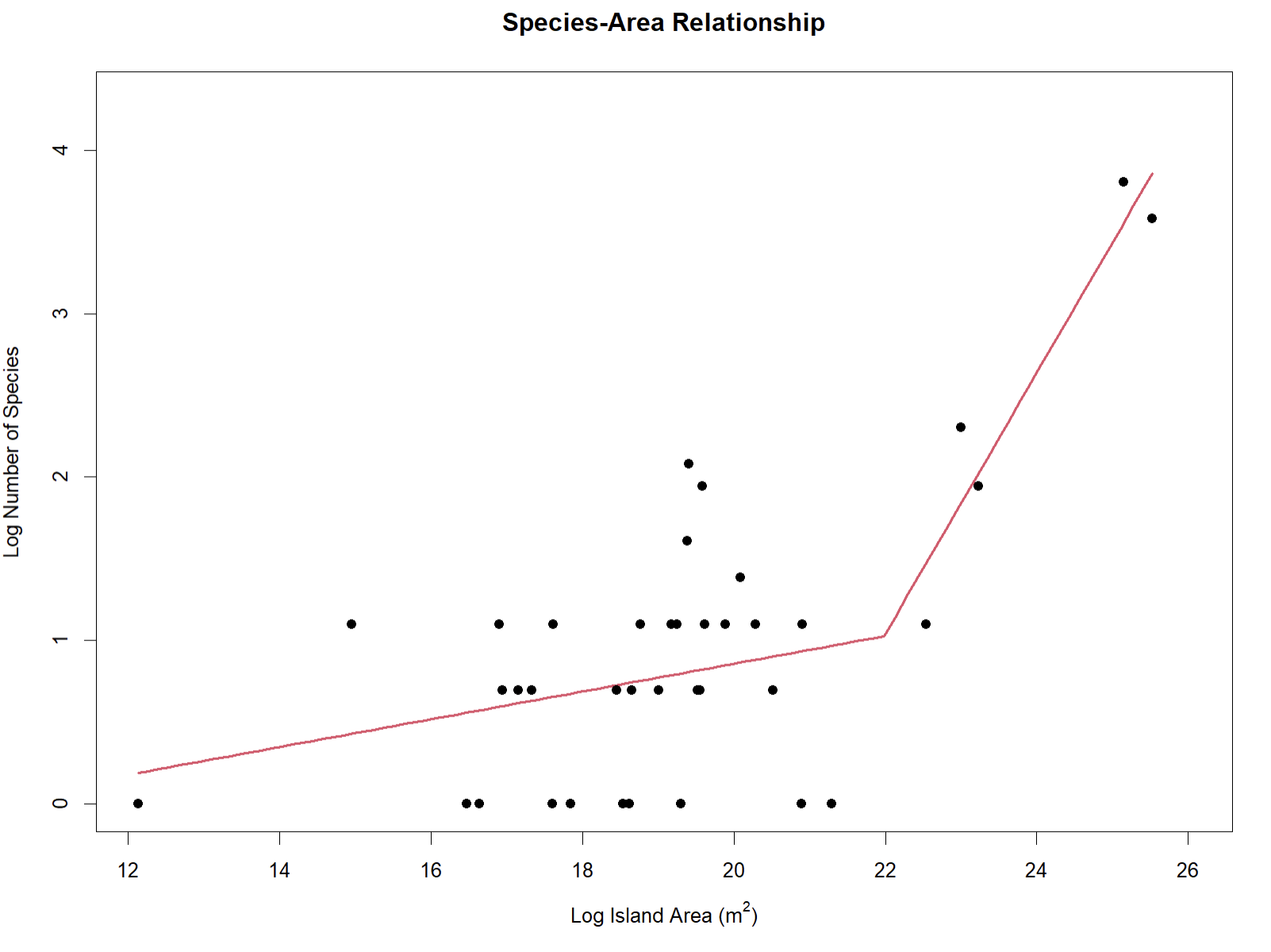
The ssarp::create_SAR() function will also output the
summary for the best-fit model for the data (displayed above).