Introduction
The ssarp R package has two main goals: create species-area relationships (SARs) when occurrence records are given as input, and create speciation-area reltionships (SpARs) when occurrence records and a phylogeny associated with the taxa of interest are given as input.
The observation that species richness increases with increasing area is a fundamental law of ecology, and a disruption in this relationship may be associated with habitat loss, habitat fragmentation, and increasing numbers of non-native species. Creating SARs for island-dwelling species helps researchers understand how trends in biodiversity across archipelagos are changing due to these effects.
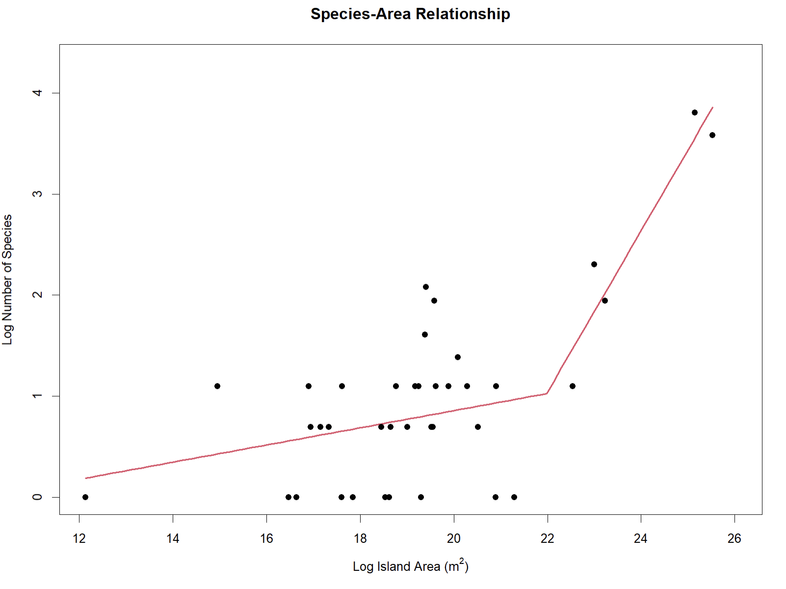
Creating SpARs, which plot speciation rates against the area of the island on which the associated species live, for the same island-dwelling species allows researchers to further explore drivers of biodiversity across archipelagos.
The creation of both of these relationships requires occurrence records for the taxa of interest. In addition, learning how to restrict these occurrence records to a specific geographic area is important for creating SARs and SpARs for a particular archipelago.
In this vignette, we will explore different options for gathering occurrence records using the rgbif package, which allows us to access data on GBIF (Global Biodiversity Information Facility) through the use of the GBIF API. These records can then be used in ssarp’s workflow to create SARs and create SpARs.
Here, we will discuss the following main topics:
- How to obtain a taxon key with
rgbiffor use in querying GBIF’s database of occurrence records - How to use
rgbif::occ_download()to obtain occurrence records for the taxon of interest - How to use
rgbif::occ_search()to obtain occurrence records for the taxon of interest - How to restrict occurrence records to a specific geographic range
using WKT geometry with
rgbif::occ_download()andrgbif::occ_search() - A suggestion for curating occurrence records from GBIF
Obtaining a Taxon Key
In order to access data from GBIF, we must first determine the unique
identifying key associated with the taxon of interest. We will use the
rgbif::name_suggest() function to find this key. To
illustrate the use of rgbif::occ_download(), we will focus
on the lizard species Anolis allisoni.
Please note that creating a SAR or SpAR for one species is not informative. This example focuses on one species to reduce the time for downloading occurrence records.
library(rgbif)

# Taxon query
query <- "Anolis allisoni"
# Taxon rank
rank <- "Species"

rgbif::name_suggest(q = query, rank = rank)
## Records returned [1]
## No. unique hierarchies [0]
## Args [q=Anolis allisoni, limit=100, rank=Species, fields1=key,
## fields2=canonicalName, fields3=rank]
## # A tibble: 1 × 3
## key canonicalName rank
## <int> <chr> <chr>
## 1 2467262 Anolis allisoni SPECIESThe rgbif::name_suggest() function will return a tibble
with taxa that closely match the query, along with their associated
keys. The name in the first row is the best match that
rgbif::name_suggest() found. The first row is the exact
correct taxon, so we will use this key to download occurrence records
from GBIF.
First, let’s save the key as a variable for use in the call to download data.
# Re-run name_suggest() call to save table
suggestions <- rgbif::name_suggest(q = query, rank = rank)

# The correct key is the first element in the first row
key <- as.numeric(suggestions$data[1,1])

# Print key
key
## [1] 2467262Downloading Occurrence Records Using occ_download()
Next, we can use rgbif::occ_download() or
rgbif::occ_search() to gather occurrence records for the
taxon of interest (Anolis allisoni).
The rgbif::occ_download() function is much more robust
than the rgbif::occ_search() function, as the
rgbif::occ_download() function does not have a limit to the
number of occurrence records returned, while the
rgbif::occ_search() function does. In addition, the
rgbif::occ_download() function creates a record of your
downloaded dataset with an associated DOI for proper citation in your
publications that utilize this data (found in the Downloads tab on
your GBIF User page).
The rgbif::occ_download() function requires the user to
have a GBIF account to use it, so
please follow the instructions here to set your GBIF username and
password in your R environment before continuing with this
vignette.
Once your GBIF credentials are added to your .Renviron file, you can
run rbif::occ_download() as written below. Please also
reference the
official vignette associated with this function to learn more
details.
The rgbif::occ_download() call includes the following
elements:
-
pred("taxonKey", key): The taxon key for Anolis allisoni that we saved above. -
pred("hasCoordinate", TRUE): Ensures that all returned records have an associated GPS coordinate. -
pred("hasGeospatialIssue", FALSE): Ensures that none of the returned records have a known geospatial issue. -
format = "DWCA": The most data-rich return format for the data. Contains information necessary for downstream ssarp functions.
download_key <- rgbif::occ_download(pred("taxonKey", key),
                                    pred("hasCoordinate", TRUE),
                                    pred("hasGeospatialIssue", FALSE),
                                    format = "DWCA")
The download_key object now contains a unique identifier
for your download. We can run
occ_download_wait(download_key) to receive an update about
the status of your download. Once the download has completed, the status
will read “succeeded.” Please note that your download may take longer
than the time limit for receiving active updates with
rgbif::occ_download_wait(), which will result in a
curl error that states Timeout was reached.
This does not mean that your download failed! When in doubt, check the Downloads tab on your GBIF
User page.
Now that the download has succeeded, the
rgbif::occ_download_get() function will allow us to
download the data as a .zip file into the current working
directory. This file is then piped into
rgbif::occ_download_import() to import the occurrence data
into the current R Environment as the dat object.
dat <- rgbif::occ_download_get(download_key) %>%
  rgbif::occ_download_import()

# Print first 5 lines of dat
head(dat)
## # A tibble: 6 × 225
## gbifID accessRights bibliographicCitation language license modified publisher references rightsHolder
## <int64> <chr> <chr> <chr> <chr> <dttm> <lgl> <chr> <chr> ##
## 1 812099598 "" "" "" CC_BY_N… 2024-12-20 18:02:42 NA http://mc… President a…
## 2 812099597 "" "" "" CC_BY_N… 2024-12-20 16:17:35 NA http://mc… President a…
## 3 812099596 "" "" "" CC_BY_N… 2024-12-20 18:01:51 NA http://mc… President a…
## 4 812099594 "" "" "" CC_BY_N… 2024-12-20 16:17:35 NA http://mc… President a…
## 5 812099593 "" "" "" CC_BY_N… 2024-12-20 18:01:51 NA http://mc… President a…
## 6 812099592 "" "" "" CC_BY_N… 2024-12-20 16:17:35 NA http://mc… President a…
## # ℹ 216 more variables: type <chr>, institutionID <chr>, collectionID <chr>, datasetID <chr>, institutionCode <chr>,
## # collectionCode <chr>, datasetName <chr>, ownerInstitutionCode <chr>, basisOfRecord <chr>,
## # informationWithheld <chr>, dataGeneralizations <lgl>, dynamicProperties <chr>, occurrenceID <chr>,
## # catalogNumber <chr>, recordNumber <chr>, recordedBy <chr>, recordedByID <chr>, individualCount <int>,
## # organismQuantity <dbl>, organismQuantityType <chr>, sex <chr>, lifeStage <chr>, reproductiveCondition <lgl>,
## # caste <lgl>, behavior <lgl>, vitality <chr>, establishmentMeans <chr>, degreeOfEstablishment <lgl>,
## # pathway <lgl>, georeferenceVerificationStatus <chr>, occurrenceStatus <chr>, preparations <chr>, …
## # ℹ Use `colnames()` to see all variable namesThe dat object is now ready to be used with the rest of
the ssarp pipeline!
Downloading Occurrence Records Using occ_search()
While rgbif::occ_download() is the optimal method for
gathering occurrence data from GBIF, the
rgbif::occ_search() function is very useful for quick
downloads that allow the user to explore occurrence records before
committing to downloading a full dataset.
In this example, we will download the first 1000 records for the entire Anolis genus on GBIF.
Similar to the rgbif::occ_download() example, we will
start by finding the taxon key associated with the Anolis
genus.
query <- "Anolis"
rank <- "Genus"

suggestions <- rgbif::name_suggest(q = query, rank = rank)

# The correct key is the first element in the first row
key <- as.numeric(suggestions$data[1,1])

# Print key
key
## [1] 8782549Next, we will use the rgbif::occ_search() function to
obtain the first 1000 occurrence records for Anolis from
GBIF.
The rgbif::occ_search() call includes the following
elements:
-
taxonKey: The taxon key for Anolis that we saved above. -
hasCoordinate = TRUE: Ensures that all returned records have an associated GPS coordinate. -
limit: The number of records returned.
# Limit for number of records returned
limit <- 1000

occurrences <- rgbif::occ_search(taxonKey = key,
                                 hasCoordinate = TRUE,
                                 limit = limit)

# The occurrences object is a list including metadata
# Access the occurrence records itself through:
dat <- occurrences$data

# Print first 5 rows of dat
head(dat)
## # A tibble: 6 × 10⁵
## key scientificName decimalLatitude decimalLongitude issues datasetKey publishingOrgKey installationKey
## <chr> <chr> <dbl> <dbl> <chr> <chr> <chr> <chr>
## 1 5006700320 Anolis sagrei Duméri… 25.8 -80.1 cdc,c… 50c9509d-… 28eb1a3f-1c15-4… 997448a8-f762-…
## 2 5006700950 Anolis lineatus Daud… 12.3 -69.0 cdc,c… 50c9509d-… 28eb1a3f-1c15-4… 997448a8-f762-…
## 3 5006703032 Anolis sagrei Duméri… 26.4 -80.2 cdc,c… 50c9509d-… 28eb1a3f-1c15-4… 997448a8-f762-…
## 4 5006714560 Anolis carolinensis … 30.4 -87.5 cdc,c… 50c9509d-… 28eb1a3f-1c15-4… 997448a8-f762-…
## 5 5006714725 Anolis sagrei Duméri… 26.3 -80.1 cdc,c… 50c9509d-… 28eb1a3f-1c15-4… 997448a8-f762-…
## 6 5006715278 Anolis carolinensis … 33.1 -117. cdc,c… 50c9509d-… 28eb1a3f-1c15-4… 997448a8-f762-…
## # ℹ 97 more variables: hostingOrganizationKey <chr>, publishingCountry <chr>, protocol <chr>, lastCrawled <chr>,
## # lastParsed <chr>, crawlId <int>, projectId <chr>, basisOfRecord <chr>, occurrenceStatus <chr>, taxonKey <int>,
## # kingdomKey <int>, phylumKey <int>, classKey <int>, familyKey <int>, genusKey <int>, speciesKey <int>,
## # acceptedTaxonKey <int>, acceptedScientificName <chr>, kingdom <chr>, phylum <chr>, family <chr>, genus <chr>,
## # species <chr>, genericName <chr>, specificEpithet <chr>, taxonRank <chr>, taxonomicStatus <chr>,
## # iucnRedListCategory <chr>, dateIdentified <chr>, coordinateUncertaintyInMeters <dbl>, continent <chr>,
## # stateProvince <chr>, year <int>, month <int>, day <int>, eventDate <chr>, startDayOfYear <int>, …The dat object is now ready to be used with the rest of
the ssarp pipeline for further exploration! If you would like
to use this data in a publication, please consider using
rgbif::occ_download() instead so that there is a DOI
automatically associated with the data.
If you must use data obtained through
rgbif::occ_search() in a publication, you must create a
Derived Dataset. The ssarp::get_sources() function helps
users create a dataframe of dataset keys and the number of occurrence
records associated with each key, which is necessary for uploading a
Derived Dataset.
Find the definition of a Derived Dataset here and more information about their creation here.
The ssarp::get_sources() function may be used as seen
below:
source_df <- ssarp::get_sources(dat)

# Print first 5 lines of source_df
head(source_df)
## datasetKey n
## 1 50c9509d-22c7-4a22-a47d-8c48425ef4a7 997
## 2 8a863029-f435-446a-821e-275f4f641165 3Restricting Occurrence Records Using Geometry
When using rgbif::occ_download() and
rgbif::occ_search(), the user can specify a well-known text
(WKT) representation of geometry to restrict the geographic location of
the returned occurrence records. The rgbif package requires
a counter-clockwise winding order for WKT.
I find it helpful to think about WKT polygons in this way: imagine a polygon around your geographic area of interest and pick one of the corners as a starting point. The order of points in WKT format should follow counter-clockwise from the corner you picked first, and the final entry in the WKT string needs to be the same as the first entry. Additionally, while GPS points are typically represented in “latitude, longitude” format, WKT expects them in “longitude latitude” format with commas separating the points rather than individual longitude and latitude values.
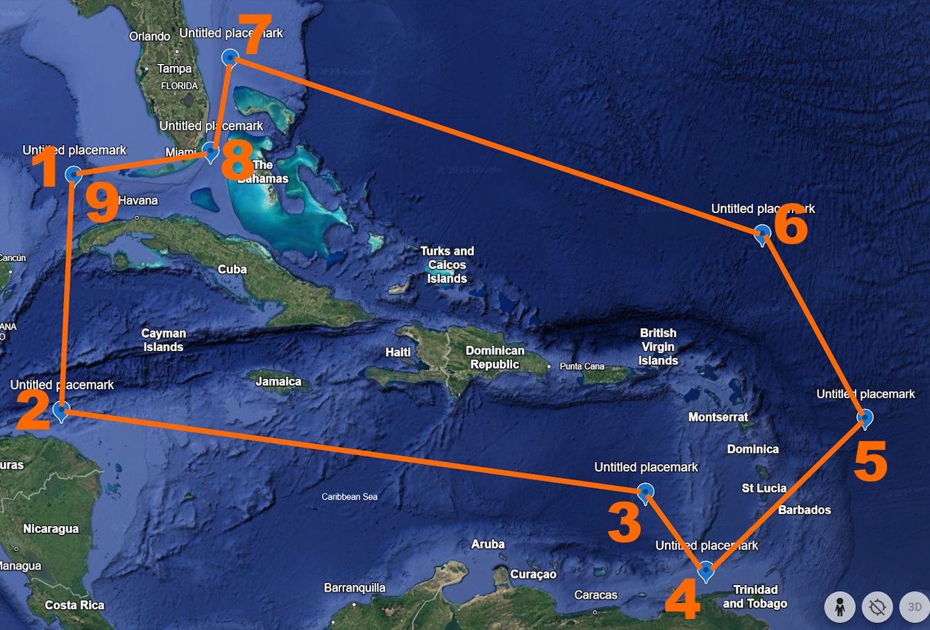
For a visual example, here is a polygon situated around Caribbean islands (Figure 1).
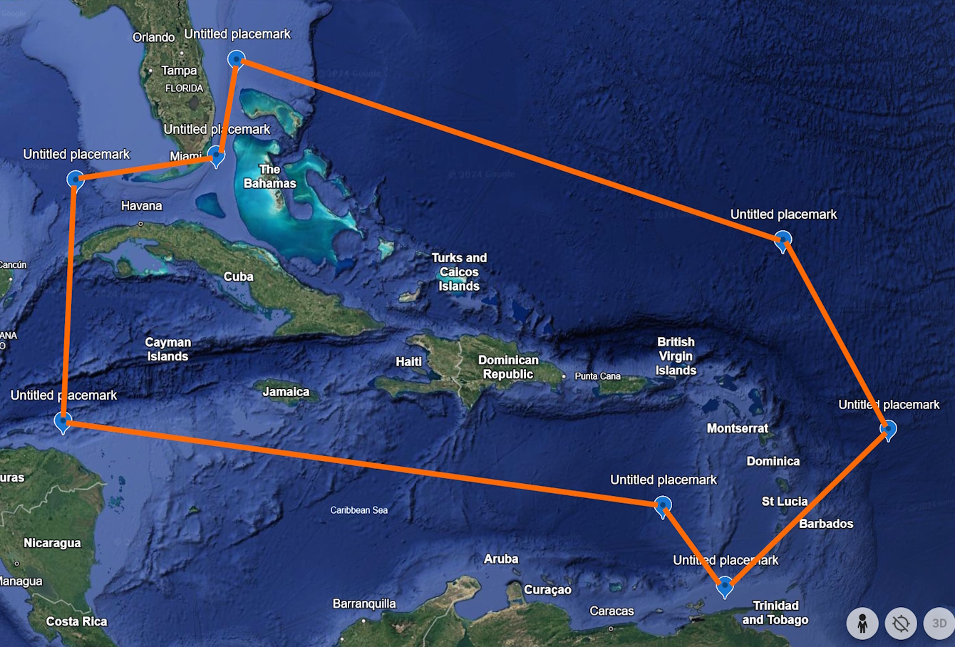
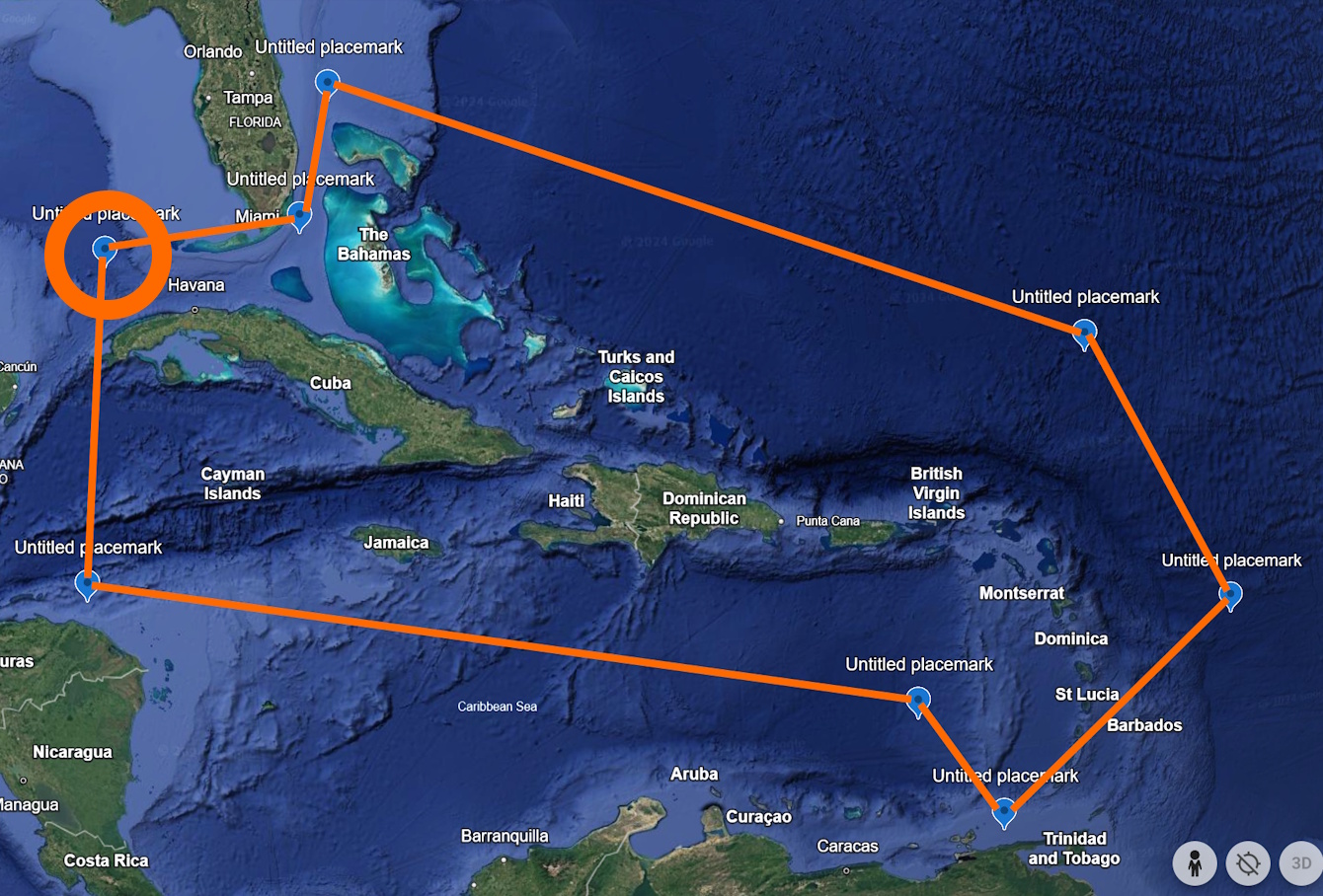
The WKT polygon for this example is ‘POLYGON((-84.8 23.9, -84.7 16.4, -65.2 13.9, -63.1 11.0, -56.9 15.5, -60.5 21.9, -79.3 27.8, -79.8 24.8, -84.8 23.9))’. The first point, normally represented by “23.9, -84.8” but written as “-84.8 23.9” for WKT, is circled in orange in Figure 2.
Then, the next point, normally represented by “16.4, -84.7” but written as “-84.7 16.4” for WKT, follows counter-clockwise from the first one (circled in Figure 3).
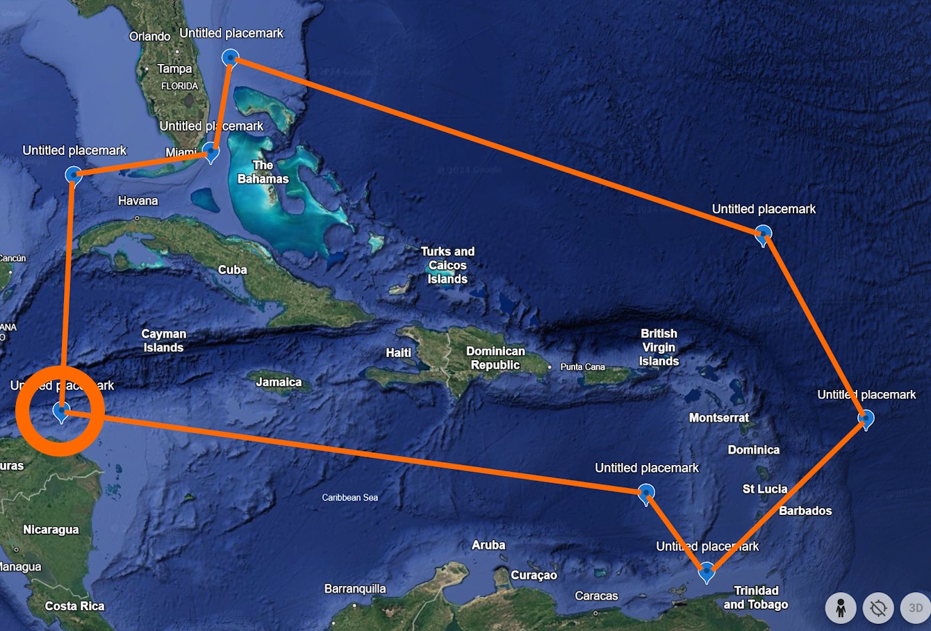
The rest of the points then follow in the order labeled in orange numbers in Figure 4. Make sure to close the polygon by ending the WKT string with the same point that you started with (“-84.8 23.9” in this case, represented by both 1 and 9 on Figure 4).
WKT polygons may be used in both rgbif::occ_download()
and rgbif::occ_search() as seen below. Please note that
variables created earlier in this document are referenced here:
# occ_download() example
download_key <- rgbif::occ_download(pred("taxonKey", key),
                              pred("hasCoordinate", TRUE),
                              pred("hasGeospatialIssue", FALSE),
                              pred_within('POLYGON((-84.8 23.9, -84.7 16.4, -65.2 13.9, -63.1 11.0, -56.9 15.5, -60.5 21.9, -79.3 27.8, -79.8 24.8, -84.8 23.9))'),
                              format = "DWCA")

# occ_search() example
occurrences <- rgbif::occ_search(taxonKey = key,
                                hasCoordinate = TRUE,
                                limit = limit,
                                geometry = 'POLYGON((-84.8 23.9, -84.7 16.4, -65.2 13.9, -63.1 11.0, -56.9 15.5, -60.5 21.9, -79.3 27.8, -79.8 24.8, -84.8 23.9))')
Curating GBIF Occurrence Records
Occurrence records returned from rgbif::occ_download()
and rgbif::occ_search() might include uninformative points.
For example, GPS points associated with occurrence records might
represent a location in the middle of the ocean when they were meant to
represent a location on an island. The ssarp::find_land()
function helps remedy this particular problem, but further data curation
might be necessary. The
CoordinateCleaner R package is an excellent resource for further
curating data downloaded from GBIF.
CoordinateCleaner sometimes flags valid records on small
islands as invalid because of buffer settings. Cross-referencing these
flagged records with the dataframe returned by
ssarp::find_land() is a great way to ensure that the user
is incorporating all valid records in their analyses.