Construct a Speciation-Area Relationship with ssarp
Source:vignettes/Create_SpAR.Rmd
Create_SpAR.RmdIntroduction
A speciation-area relationship (SpAR) plots speciation rates against the area of the island on which the associated species live. This vignette, which covers how to create a SpAR using the ssarp package, uses knowledge and data generated from the vignette describing the creation of species-area relationships. Code relevant to generating the necessary data for this SpAR example from the species-area relationship (SAR) vignette will be included here, but the reader is encouraged to read the SAR vignette for additional details.
In this vignette, we will create a SpAR for the lizard genus Anolis, as a continuation of the SAR vignette.
Generate Occurrence Data
First, we will generate the “nocont_dat” object from the SAR vignette, which includes occurrence records and their associated island names and areas for Anolis lizards that live on Caribbean islands.
library(rgbif)
library(ssarp)

# Get the GBIF key for the Anolis genus
query <- "Anolis"
rank <- "Genus"

suggestions <- rgbif::name_suggest(q = query, rank = rank)

key <- as.numeric(suggestions$data[1,1])

# Get data for Anolis from GBIF from islands in the Caribbean
limit <- 10000
occurrences <- rgbif::occ_search(taxonKey = key,
                                hasCoordinate = TRUE,
                                limit = limit,
                                geometry = 'POLYGON((-84.8 23.9, -84.7 16.4, -65.2 13.9, -63.1 11.0, -56.9 15.5, -60.5 21.9, -79.3 27.8, -79.8 24.8, -84.8 23.9))')

dat <- occurrences$data

# Find land mass names
land_dat <- ssarp::find_land(occurrences = dat)

# Use the land mass names to get their areas
area_dat <- ssarp::find_areas(occs = land_dat)

# Remove continents from the filtered occurrence record dataset
nocont_dat <- ssarp::remove_continents(occs = area_dat)
Calculate Speciation Rates
The “nocont_dat” object created above can be used with a phylogenetic tree to create a SpAR. This step in the ssarp workflow enables the user to determine whether the breakpoint in the SAR corresponds with a threshold for island size at which in situ speciation occurs (see Losos and Schluter 2000).
The phylogenetic tree for Anolis that we will use in this example is a trimmed version of the tree used by Patton et al. (2021). This trimmed tree only includes anoles found on islands in the Caribbean. In order to read the tree, we must use the ape R package.
library(ape)

tree <- read.tree(system.file("extdata",
                              "Patton_Anolis_trimmed.tree",
                              package = "ssarp"))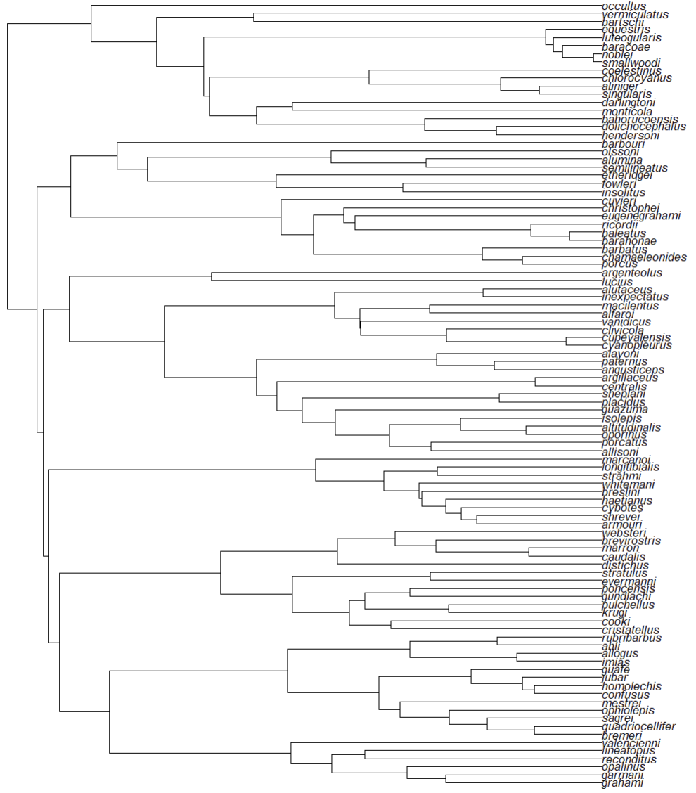
Now that we have a phylogenetic tree, we can estimate tip speciation rates for use in our speciation-area relationship. ssarp includes three methods for estimating tip speciation rates: BAMM (Rabosky 2014), the lambda calculation for crown groups from Magallόn and Sanderson (2001), and DR (Jetz et al. 2012).
The ssarp::estimate_BAMM function requires a
bammdata object as input, which must be created using the
BAMMtools package (Rabosky et al. 2014) after the user
completes a BAMM analysis. This object includes tip speciation rates by
default in the “meanTipLambda” list element, which ssarp
accesses to add the appropriate tip speciation rates for each species to
the occurrence record dataframe.
DR stands for “diversification rate,” but it is ultimately a better
estimation of speciation rate than net diversification (Belmaker and
Jetz 2015; Quintero and Jetz 2018) and returns results similar to BAMM’s
tip speciation rate estimations (Title and Rabosky 2019). The
ssarp::estimate_DR function returns the values obtained
from running an adapted version of the “DR_statistic” function from Sun
and Folk (2020).
In addition to tip speciation rates, SSARP includes a function for
calculating the speciation rate for a clade from Magallόn and Sanderson
(2001). The ssarp::estimate_speciation function uses the
ape::subtrees function (Paradis and Schliep 2019) to
generate all possible subtrees from the user-provided phylogenetic tree
that corresponds with the taxa of interest for the SpAR. Then, species
in the provided occurrence records generated from previous steps in the
ssarp workflow are grouped by island. For each group of
species that comprise an island, the number of subtrees that represent
that group of species and the root age of each subtree is recorded,
along with the name and area of the island. The speciation rate for each
subtree is then calculated following Equation 4 in Magallόn and
Sanderson (2001). If an island includes multiple subtrees, the island
speciation rate is the average of the calculated speciation rates. This
average is calculated when the SpAR is plotted.
In this example, we will use the lambda calculation for crown groups
from Magallόn and Sanderson (2001) through the
ssarp::estimate_MS() function. The “label_type” parameter
in this function tells ssarp whether the tip labels on the
given tree include the full species name (binomial) or just the specific
epithet (epithet).
# Calculate tip speciation rates using the lambda calculation for crown groups from Magallόn and Sanderson (2001)
speciation_occurrences <- ssarp::estimate_MS(tree = tree, label_type = "epithet", occurrences = nocont_dat)
The “speciation_occurrences” object is a dataframe containing island
areas with their corresponding speciation rate as estimated by the
ssarp::estimate_MS() function.
Create Speciation-Area Relationship
Next, we will use the “speciation_occurrences” object with the
ssarp::create_SpAR() function to create a SpAR. Just like
the ssarp::create_SAR() function, the
ssarp::create_SpAR() function creates multiple regression
objects with breakpoints up to the user-specified “npsi” parameter. For
example, if “npsi” is two, ssarp::create_SpAR() will
generate regression objects with zero (linear regression), one, and two
breakpoints. The function will then return the regression object with
the lowest AIC score. The “npsi” parameter will be set to one in this
example. Note that if linear regression (zero breakpoints) is
better-supported than segmented regression with one breakpoint, the
linear regression will be returned instead.
ssarp::create_SpAR(occurrences = speciation_occurrences, npsi = 1)##
## ***Regression Model with Segmented Relationship(s)***
##
## Call:
## segmented.lm(obj = linear, seg.Z = ~x, npsi = 1, control = segmented::seg.control(display = FALSE))
##
## Estimated Break-Point(s):
## Est. St.Err
## psi1.x 19.924 1.036
##
## Coefficients of the linear terms:
## Estimate Std. Error t value Pr(>|t|)
## (Intercept) 1.364e-12 2.233e-02 0.000 1
## x -8.298e-14 1.227e-03 0.000 1
## U1.x 5.712e-03 2.150e-03 2.656 NA
##
## Residual standard error: 0.01069 on 32 degrees of freedom
## Multiple R-Squared: 0.3968, Adjusted R-squared: 0.3403
##
## Boot restarting based on 6 samples. Last fit:
## Convergence attained in 2 iterations (rel. change 2.5337e-14)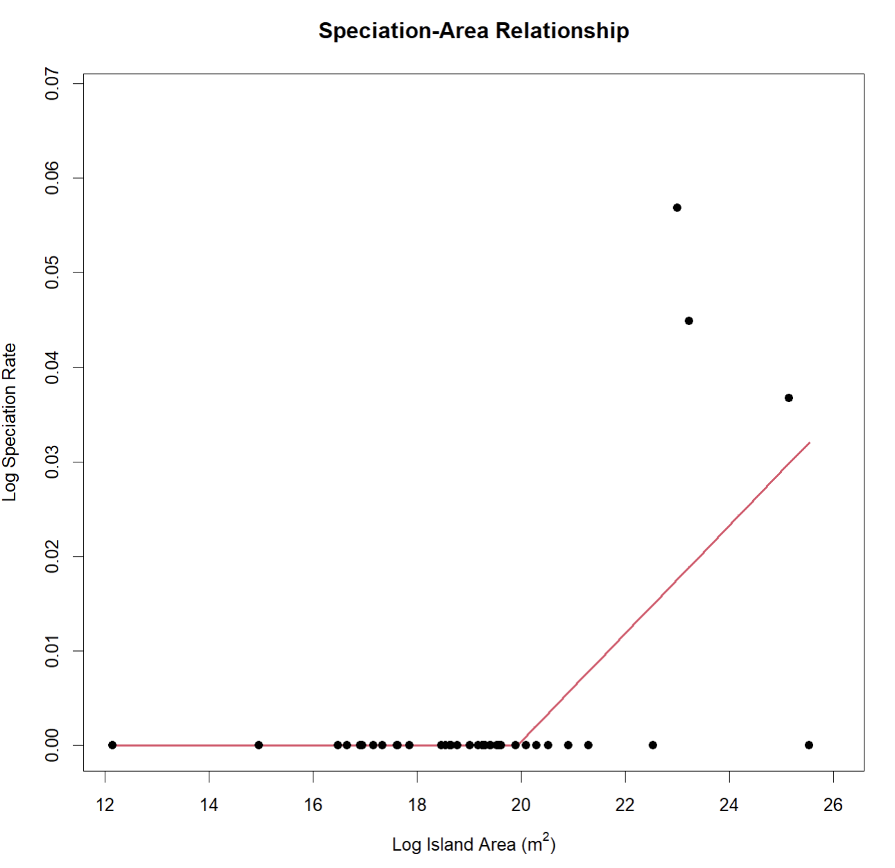
You will notice that two of the largest islands have a speciation
rate of zero in this example. This very likely occurred because the
calculation for speciation rate in Magallόn and Sanderson (2001) that
ssarp::estimate_MS() uses is based on monophyly, which can
be disrupted on islands with non-native species occurrence records. When
using the ssarp::estimate_MS() function to estimate
speciation rates for a SpAR, it is incredibly important to manually
filter the returned occurrence records to remove non-native species.
Literature Cited
- Belmaker, J., & Jetz, W. (2015). Relative roles of ecological and energetic constraints, diversification rates and region history on global species richness gradients. Ecology Letters, 18: 563–571.
- Jetz, W., Thomas, G.H., Joy, J.B., Hartmann, K., & Mooers, A.O. (2012). The global diversity of birds in space and time. Nature, 491: 444-448.
- Losos, J.B. & Schluter, D. (2000). Analysis of an evolutionary species-area relationship. Nature, 408: 847-850.
- Magallόn, S. & Sanderson, M.J. (2001). Absolute Diversification Rates in Angiosperm Clades. Evolution, 55(9): 1762-1780.
- Paradis, E. & Schliep, K. (2019). ape 5.0: an environment for modern phylogenetics and evolutionary analyses in R. Bioinformatics, 35: 526-528.
- Patton, A.H., Harmon, L.J., del Rosario Castañeda, M., Frank, H.K., Donihue, C.M., Herrel, A., & Losos, J.B. (2021). When adaptive radiations collide: Different evolutionary trajectories between and within island and mainland lizard clades. PNAS, 118(42): e2024451118.
- Quintero, I., & Jetz, W. (2018). Global elevational diversity and diversification of birds. Nature, 555, 246–250.
- Rabosky, D.L. (2014). Automatic Detection of Key Innovations, Rate Shifts, and Diversity-Dependence on Phylogenetic Trees. PLOS ONE, 9(2): e89543.
- Rabosky, D.L., Grundler, M., Anderson, C., Title, P., Shi, J.J., Brown, J.W., Huang, H., & Larson, J.G. (2014), BAMMtools: an R package for the analysis of evolutionary dynamics on phylogenetic trees. Methods in Ecology and Evolution, 5: 701-707.
- Sun, M. & Folk, R.A. (2020). Cactusolo/rosid_NCOMMS-19-37964-T: Code and data for rosid_NCOMMS-19-37964 (Version V.1.0). Zenodo. http://doi.org/10.5281/zenodo.3843441
- Title P.O. & Rabosky D.L. (2019). Tip rates, phylogenies and diversification: What are we estimating, and how good are the estimates? Methods in Ecology and Evolution. 10: 821–834.